Two seeds, two solitudes. By forcing one longitudinal field to vanish, Kira and Voss unlock the cylindrical Helmholtz equation — chasing Frobenius series, Bessel roots, and the boundary laws that decide which waves propagate and which die.
The metal corridor had not grown any warmer, but the silence had changed. It was no longer the empty silence of a dark tube; it was the expectant silence of a circuit waiting for a switch to close.
Behind them lay the ledger: four transverse equations, pinned entirely to two unplanted seeds — Ez and Hz — and one exchange rate, kc², holding the budget between moving forward and standing transverse. But leaving both seeds alive simultaneously was an intolerable knot. Every transverse field was pulled by two masters at once.
If we leave both alive, the equations choke on their own cross-talk. We're asking this metal throat to sing in two languages at the same instant.
Then we enforce a covenant. We silence one. Deliberately. Completely.
He held up a finger, tracing a zero into the dark air between them.
Set Hz = 0. The magnetic field loses all authority to travel forward — it is pinned flat against the cross-section, purely transverse. Only Ez is allowed to spear lengthwise down the corridor. We call that Transverse Magnetic: TM. And once we see what shape Ez takes, we flip the coin and do the mirror.
One seed at a time. Show me how the cylinder carves Ez.
This is the exact mathematical path: from the TM curl equations to the cylindrical Scalar Helmholtz PDE, through the Frobenius series expansion, the exile of the Neumann singularity, and the Bessel roots that govern cutoffs.
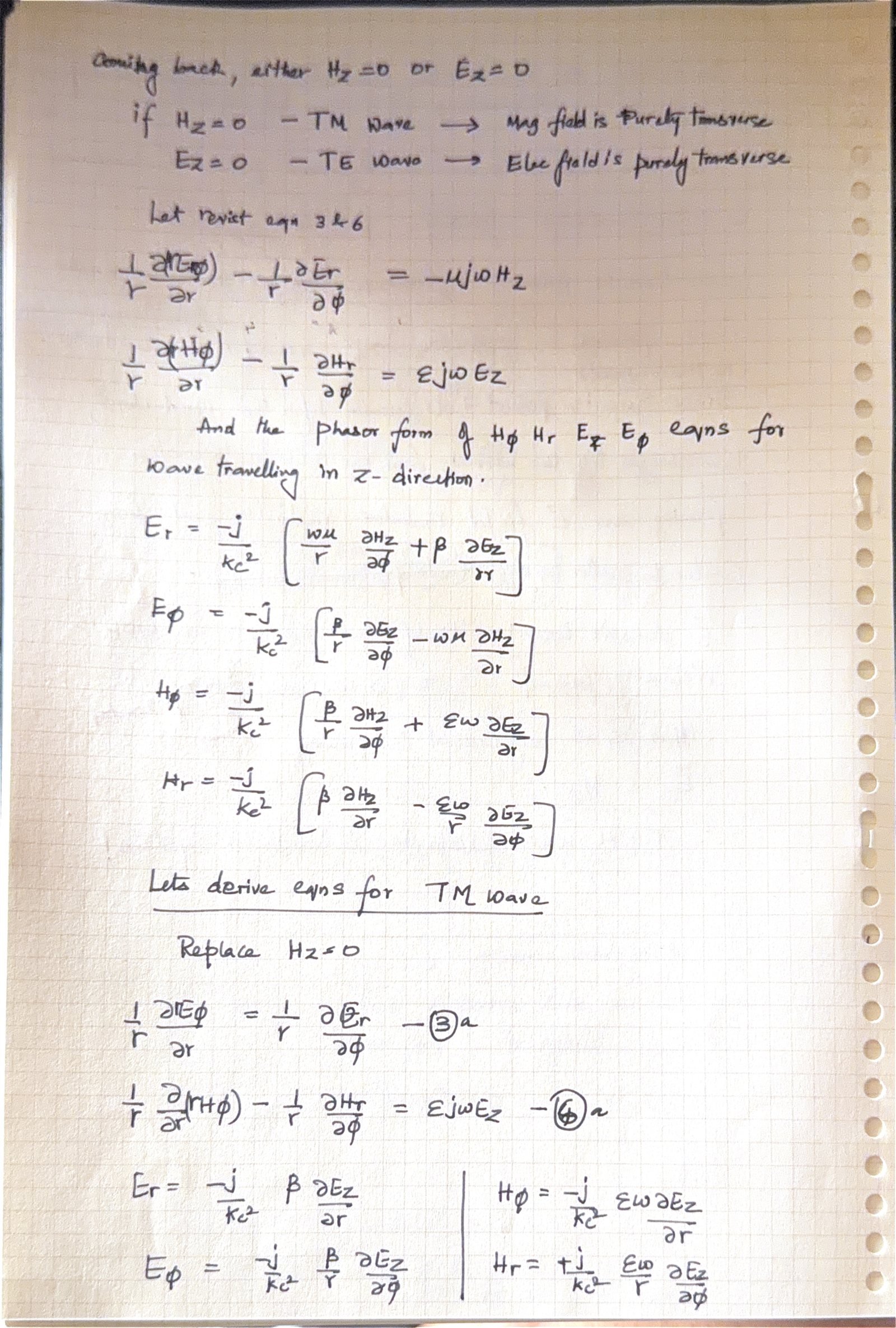
Revisiting the transverse equations from Episode 01 with the condition Hz = 0 collapses the system immediately. All terms carrying Hz vanish, leaving all four transverse components governed exclusively by the single longitudinal electric seed Ez:
To find the governing equation for Ez, we return to the z-component of Ampère's Law (Equation 6a from Episode 01):
Now, substitute our TM transverse expressions for Hφ and Hr into the left side. The radial and angular derivatives act on Ez:
Plugging these back into Equation 6a and dividing out the factor of j ε ω from both sides:
Multiplying by −kc² and moving all terms to one side reveals the iconic Scalar Helmholtz Equation in Cylindrical Coordinates:
Kira knelt beside the equation, running a finger along the curve of the radial bracket.
It's a partial differential equation. r and φ are tangled up inside the same brackets. The wave is trying to decide how many ripples it makes around the circumference while simultaneously deciding how it dies or peaks as it heads toward the metal wall.
Then we separate them. We make an ansatz: assume the field can be factored into a pure radial function R(r) and a pure azimuthal function Φ(φ). If the cylinder is uniform, the angular ripple has no business depending on radius.
He wrote out the separation hypothesis:
Substituting this product into the Helmholtz equation, dividing through by R(r) Φ(φ), and multiplying by r² forces the variables to opposite sides of an uncrossable ledger:
Look at that equality. The left side depends only on r. The right side depends only on φ. If you change radius, the right side cannot move. If you rotate angle, the left side cannot move. The only way two independent variables can equal each other across the entire cylinder is if both equal the exact same constant: n².
And why n² instead of just n? Because we know what comes out of double differentiation — harmonic sines and cosines. But what fixes n? Why can't it be 1.7 or π?
Because space closes on itself. Walk 360 degrees around this corridor: φ → φ + 2π. You arrive at the exact same physical point in space. If Φ(φ + 2π) ≠ Φ(φ), the electric field would have two different values at the exact same spot in space. Nature forbids that ambiguity. n must be an integer: n = 0, 1, 2, 3...
Setting the radial half equal to n² and multiplying out produces the legendary Bessel Differential Equation:
Because of the variable coefficient (kc² r² − n²), standard exponential solutions fail. As worked out step-by-step on pages 6–14 of the original notes, we attack this equation with the Frobenius Method of Generalized Power Series:
Substituting the power series into the differential equation and examining the lowest-order power of r yields the indicial equation:
For the positive root s = +n, matching powers of rk+n yields the recurrence relation that connects every second coefficient:
All odd coefficients C1, C3, C5 vanish. Computing the even terms sequentially generates the alternating series:
Voss paused his pencil on the page. The derivation had split into two classical branches.
A second-order differential equation always yields two independent solutions. The general radial solution isn't just Jn. It is a linear combination of Jn and the Neumann function Yn:
Look at what Yn does as r approaches zero. It plunges straight to negative infinity.
She pointed dead center down the metallic conduit.
The center of this pipe is empty air. There is no wire at r = 0, no line of infinite charge, no laser cutting a hole through the universe. If Yn is allowed to live, the electric field along the centerline would be infinite. It would require infinite energy to launch.
Physical realizability. The center must remain finite. Therefore, C2 = 0. The Neumann singularity is banished.
With that single stroke of physical reality, the general TM solution collapsed into its true, clean form:
We have the field shape, but kc is still an arbitrary number. To pin it down, we confront the outer conductor wall at r = a.
The boundary condition on a perfect conductor demands that the tangential electric field must perish at the metal surface:
This is the moment of quantization. kc a cannot be any continuous value; it is forced to land on the zeros of the Bessel function. We denote the m-th root of Jn as pnm:
Recalling the corridor's master exchange rate from Episode 01: kc² = ω²με − β². At the cutoff frequency fc, the wave expends all its energy purely across the cross-section and has zero budget left to move forward (β = 0):
Kira wiped chalk from her fingers, stepping back from the TM derivation.
We silenced Hz and let Ez build the cylinder. Now flip the coin. What happens when we silence Ez = 0 and let Hz rule the axis?
Transverse Electric: TE. E is pinned flat into the transverse plane. Hz satisfies the exact same cylindrical Helmholtz equation, and its radial function is also governed by Jn(kc r):
Wait. Does the wall force Hz(a) = 0 as well?
No! That is the critical asymmetry. Hz is parallel to the conducting wall. Magnetic fields parallel to a conductor don't vanish — they drive surface currents: Js = n̂ × H. Hz is free to be non-zero right at r = a!
Then what holds the boundary? What stops TE from taking any frequency it wants?
Tangential E! Look at Eφ at r = a. Eφ runs along the circular wall. That conductor forces Eφ = 0. And look at what Eφ equals in terms of Hz:
Kira's eyes lit up as she recognized the derivative:
To make Eφ zero at the wall, the derivative of Hz with respect to r must be zero! The slope has to flatten out!
For TE waves, the cutoff is not governed by the roots of Jn, but by the roots of its derivative J'n, denoted p'nm:
We now hold both keys: the zeros of Jn (for TM) and the zeros of J'n (for TE). When an electromagnetic wave of increasing frequency enters this circular waveguide, which mode is granted passage first?
| Mode | Governing Root | Root Value | Relative Cutoff (fc / fc_dominant) | Status |
|---|---|---|---|---|
| TE11 | p'11 | 1.8412 | 1.000 | ★ DOMINANT MODE (Lowest Cutoff) |
| TM01 | p01 | 2.4048 | 1.306 | First Circularly Symmetric Mode |
| TE21 | p'21 | 3.0542 | 1.659 | Quadrupole Transverse Mode |
| TE01 | p'01 | 3.8317 | 2.081 | Ultra-Low Attenuation Mode |
| TM11 | p11 | 3.8317 | 2.081 | Degenerate with TE01 |
The numbers had stopped fighting. The roots were mapped, the Bessel functions cataloged, and the hierarchy between TM and TE laid bare on the cold conduit wall. But numbers on a ledger are not yet fields in motion.
"Voss," Kira whispered, her hand hovering over the glowing conduit aperture. "These aren't just eigenvalues. They are shapes. TE11 has two lobes looping across the center. TM01 radiates outward like spokes on a glowing wheel. What does it actually look like when an RF pulse surges through this pipe in real time?"
Voss stepped up to the field-solver terminal. His fingers danced across the console, initializing the Yee cell mesh and preparing the first electromagnetic simulation pulse.
Both Parts 1 and 2 of the handwritten derivation — from the initial TM curl reduction, through the complete 14-page Frobenius series expansion and Bessel recursion, to the wall boundary conditions and TE derivative zeros — have been combined into this unified 27-page interactive archive.