The First Pulse
From Bessel's parchment to the Yee-cell lattice: uncovering spatial field topologies, the reality of overmoding, and the virtual crucible of electromagnetic simulation.
Beyond the Ink
The amber phosphor glow of the field-solver console painted long shadows against the bulkhead. On the drafting glass lay the 27 handwritten pages of Episode 02: the Frobenius series reductions, the indicial roots, and the algebraic banishment of Neumann singularities. The math was airtight. But mathematics is a blueprint, not a burning field.
"Voss, you proved the Bessel roots with chalk and caffeine. We know p'11 ≈ 1.841 and p01 ≈ 2.405. But standing inside this conduit, what actually happens when we inject a 5 gigahertz wave into the aperture? Does the field politely follow our equations, or do higher-order ghosts tear the wavefront apart?"
Voss cracked his knuckles over the terminal keyboard, initializing the 3D finite-element mesh. The wireframe cylinder materialized in holographic green: twenty-five millimeters of inner radius, five hundred millimeters of seamless, polished copper corridor along the z-axis.
"When a high-frequency wave strikes the boundary of a waveguide, it doesn't choose a single path. It attempts to excite every conceivable mode—every combination of angular and radial index (m, n)—simultaneously. The waveguide acts as a spatial sieve. A high-pass filter forged in pure geometry."
"And if we feed it a frequency high enough to wake up more than one mode at once...?"
"Overmoding. Spatial beating. Interference fringes racing along the axis like phantom pulses. Before we hit 'Solve', let's map the living topology of these modes on the glass."
The Coordinates of Life and Death
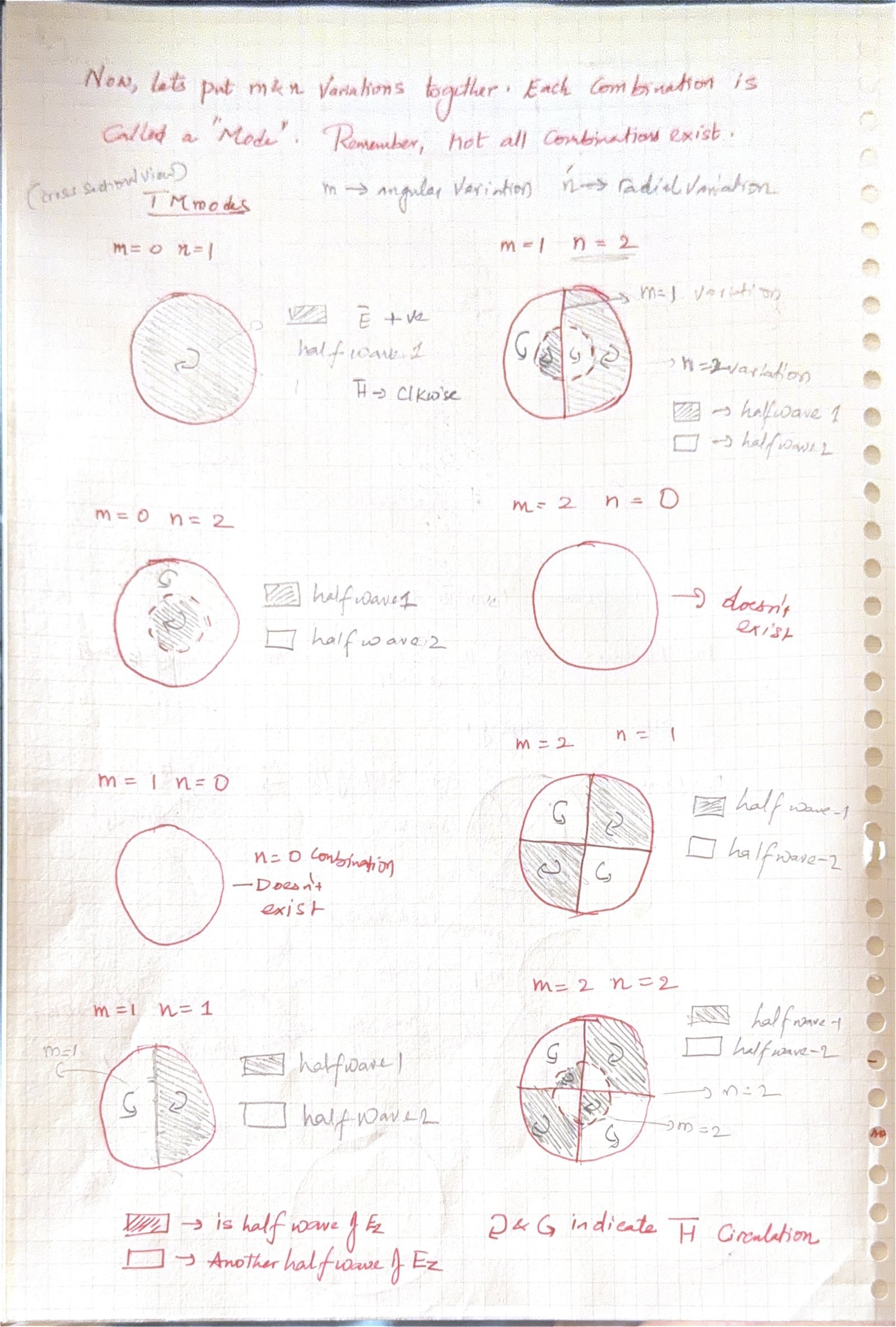
Kira pulled up the cross-sectional view of the circular aperture. The mode indices (m, n) were not abstract integers—they were the physical count of geometric nodes across the pipe:
m (Angular Index): Represents the number of full azimuthal cycles around the pipe circumference. It dictates the number of diametral nodal planes.
n (Radial Index): Represents the number of field zeros (nodes) along the radial direction from the centerline (r = 0) to the conducting outer wall (r = a).
Note on Existence: The combination n = 0 never exists in circular waveguides! Because the boundary requires a physical zero crossing at the wall, at least one radial variation must occur (n ≥ 1).
Electric field Ez peaks fiercely at the centerline (r = 0) and smoothly drops to zero at the wall. The magnetic field H circulates in pure clockwise loops around the axis.
Electric field lines loop across the transverse diameter like dipolar arches. Magnetic circulation is split into two opposing halves. Wall boundary condition clamps J'1(kca) = 0 (an antinode!).
TM02 has an inner glowing core surrounded by a reversed outer ring. TM11 splits into two angular quadrants with alternating polarity.
Four distinct quadrants of alternating H circulation and transverse E field loops. Requires significantly higher excitation frequencies to ignite.
"Look at the boundary condition difference between them! In TM modes, the wall is a node (Ez = 0, Dirichlet condition via Jm(kca) = 0). But in TE modes, the wall is an antinode (∂Hz / ∂r = 0, Neumann condition via J'm(kca) = 0). That's why the rings for TE and TM modes occur at completely different radii!"
"Exactly. And because the waveguide operates as a high-pass filter, any mode whose calculated cutoff frequency fc sits above our incoming carrier frequency is choked out into an evanescent wave—its amplitude dying exponentially within millimeters of the port."
The C-Band Verification Challenge
We specify a high-power copper circular waveguide for a C-band radar feed. Let us analytically determine every cutoff frequency, phase velocity, wave impedance, and dielectric breakdown threshold before executing the numerical simulation.
Radius: a = 25 mm = 0.025 m (Diameter: 50 mm)
Conduit Length: L = 500 mm = 0.50 m
Operating RF Frequency: f = 5.0 GHz (C-Band)
Interior Dielectric: Vacuum / Dry Air (εr = 1, μr = 1, c = 3.0 × 10⁸ m/s)
Using the Bessel function root values from our ledger (p'11 = 1.841, p01 = 2.405, p'21 = 3.054):
fc(TE11) = (c · p'11) / (2π · a) = (3.0 × 108 · 1.841) / (2π · 0.025) = 3.516 GHz
// Since fc(3.516 GHz) < 5.0 GHz → PROPAGATES (PASS)
// 2. TM01 (First Higher-Order Mode)
fc(TM01) = (c · p01) / (2π · a) = (3.0 × 108 · 2.405) / (2π · 0.025) = 4.593 GHz
// Since fc(4.593 GHz) < 5.0 GHz → PROPAGATES (PASS)
// 3. TE21 (Second Higher-Order Mode)
fc(TE21) = (c · p'21) / (2π · a) = (3.0 × 108 · 3.054) / (2π · 0.025) = 5.833 GHz
// Since fc(5.833 GHz) > 5.0 GHz → CHOKED / EVANESCENT DEATH (FAIL)
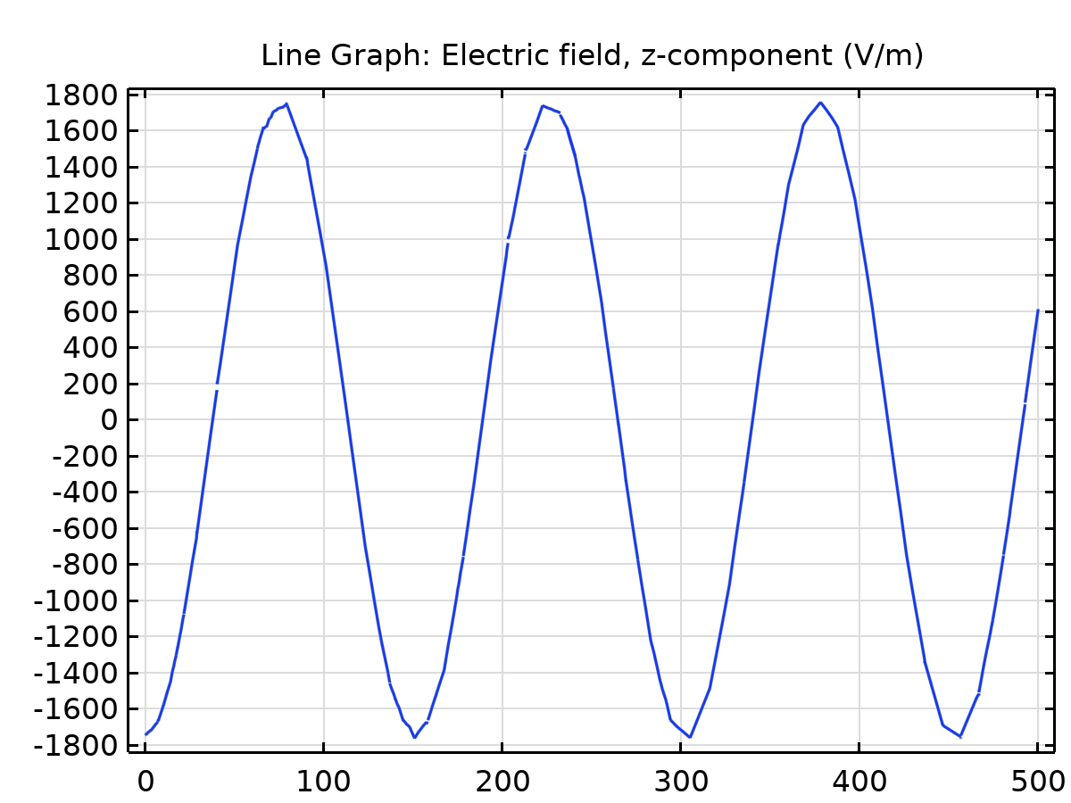
Notice that at 5.0 GHz, both TE11 and TM01 propagate simultaneously! The waveguide is overmoded. If an antenna launcher excites both modes, they will co-exist, superimpose, and beat against each other along the length of the conduit.
Waveguide phase velocity measures the velocity of a constant-phase wavefront (crest or trough) propagating axially along the tube:
// For TE11 at 5 GHz:
vp(TE11) = 3.0 × 10⁸ / √(1 - (3.516 / 5.0)2) = 3.0 × 10⁸ / √(1 - 0.4945) = 4.219 × 10⁸ m/s
// For TM01 at 5 GHz:
vp(TM01) = 3.0 × 10⁸ / √(1 - (4.593 / 5.0)2) = 3.0 × 10⁸ / √(1 - 0.8438) = 7.593 × 10⁸ m/s
"Look at that velocity discrepancy! The TM01 wavefront races at 7.593 × 10⁸ m/s—more than 2.5 times the speed of light in vacuum, and almost twice as fast as the TE11 wavefront! How does that not violate special relativity?"
"Because phase velocity carries zero information. Information and energy propagate at the group velocity vg = c · √(1 - (fc/f)2), such that vp · vg = c2. For TM01, vg crawls at barely 0.395 c. But in a linear particle accelerator, if we inject a relativistic proton into this pipe, the proton can only travel at v < c. The TM01 crest outruns the particle so violently that the accelerating field turns into a decelerating trough before the proton even moves a few centimeters! That's why accelerator engineers must deform the pipe walls with periodic copper irises to build a slow-wave structure."
In bounded waveguides, the intrinsic wave impedance differs completely from free-space impedance (η0 ≈ 377 Ω):
Z(TE11) = η0 / √(1 - (fc / f)2) = 377 / 0.7110 = 530.24 Ω
// TM Mode Impedance (Always less than free space):
Z(TM01) = η0 · √(1 - (fc / f)2) = 377 · 0.3950 = 148.95 Ω
If an engineer connects a standard 50 Ω coaxial transmission line directly to this aperture without an impedance matching transformer, catastrophic reflections and high Voltage Standing Wave Ratio (VSWR) will choke the transmission.
In dry atmospheric air, dielectric breakdown occurs when the peak local electric field reaches Ebd = 3 MV/m (3 × 10⁶ V/m), igniting destructive plasma arcing. Integrating the Poynting vector over the circular cross section yields:
Pmax(TE11) = [π a2 Ebd2 / Z(TE11)] · (1 - 1 / (p'11)2) · J12(p'11)
With p'11 = 1.841, J1(1.841) ≈ 0.5819:
Pmax(TE11) = [π · (0.025)2 · (3 × 106)2 / 530.24] · (1 - 1 / (1.841)2) · (0.5819)2 = 7.955 MW
// TM01 Power Capacity Formula:
Pmax(TM01) = [π a2 Ebd2 / (2 · Z(TM01))] · ((f / fc)2 - 1) · J12(p01)
With p01 = 2.405, J1(2.405) ≈ 0.5191:
Pmax(TM01) = [π · (0.025)2 · (3 × 106)2 / (2 · 148.95)] · ((5 / 4.593)2 - 1) · (0.5191)2 = 2.957 MW
In pure ultra-high vacuum, the theoretical field limit leaps to Emax ≈ 59.3 MV/m, enabling the conduit to handle upwards of 3.1 Gigawatts of RF power!
Executing the Field Solver
Voss switched to the COMSOL Multiphysics environment. The analytical equations had set the trap; the numerical finite element engine was about to test it.
1. Geometry: 3D Cylinder, r = 25 mm, Height h = 500 mm aligned along the z-axis.
2. Boundaries: Cylindrical outer walls set to Perfect Electric Conductor (PEC): n × E = 0. End cross-sections left open for ports.
3. Numerical Ports: Port 1 at z = 0 (excited with 1 W input power), Port 2 at z = 500 mm (absorbing receiver).
4. The Eigenvalue Mode Shift Trick: In Study Step 1 (Boundary Mode Analysis), searching blindly across infinite degrees of freedom causes slow or diverging convergence. Instead, we seed the solver with our hand-calculated effective mode index:
neff = √(1 - (fc/f)2)
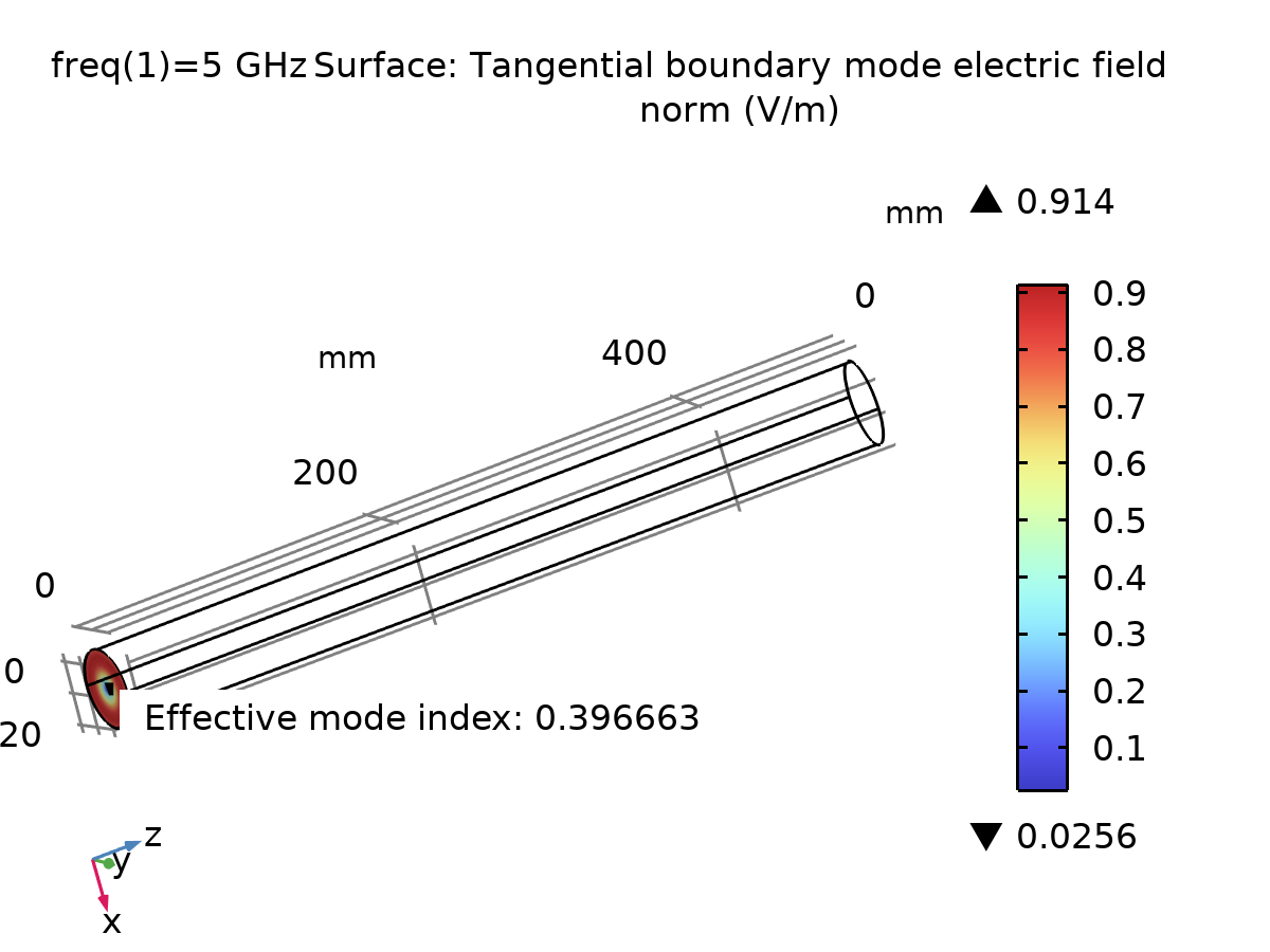
We inject neff = 0.711 for TE11, and neff = 0.395 for TM01. The eigenvalue solver converges in under 1 second!
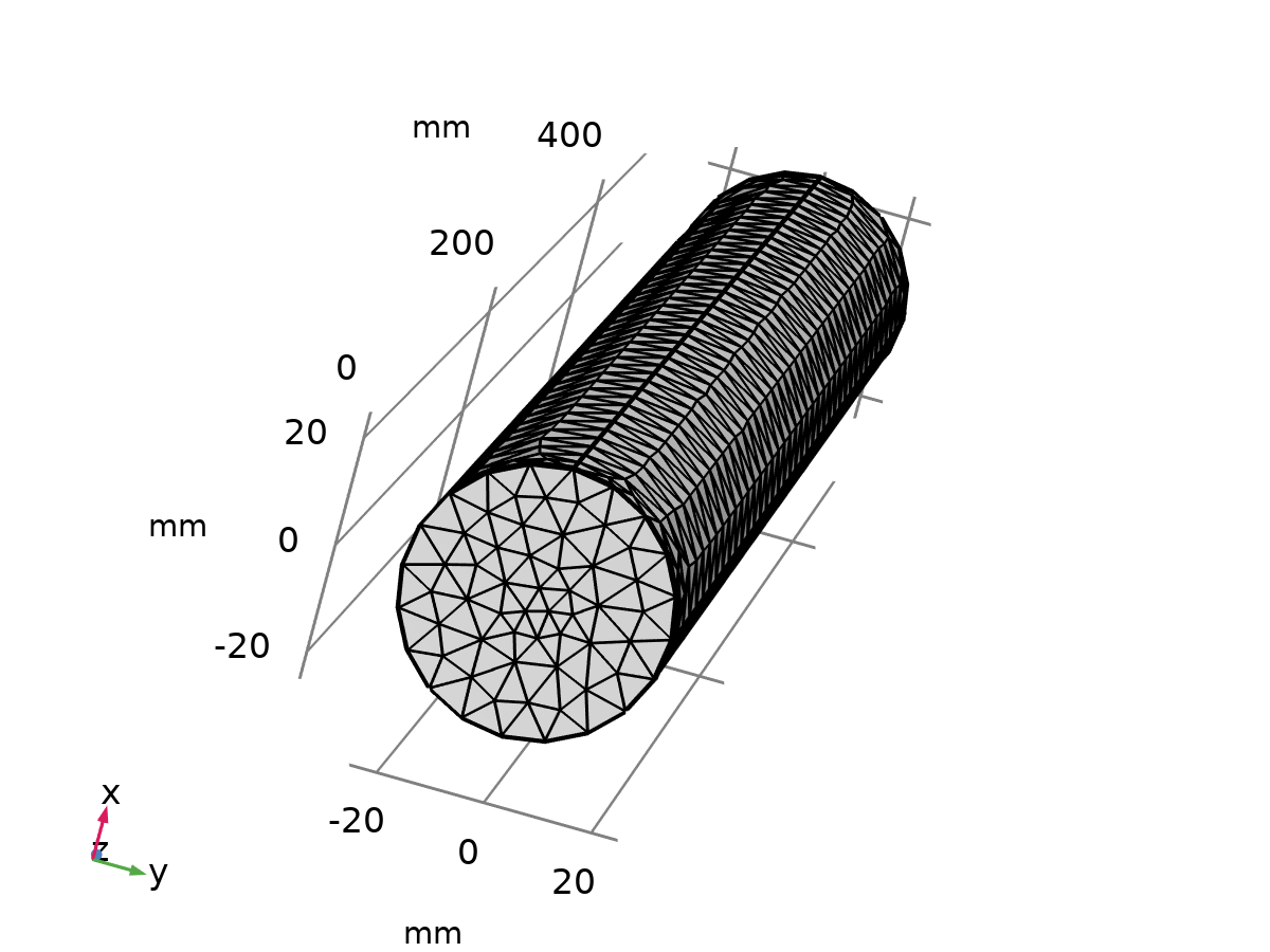
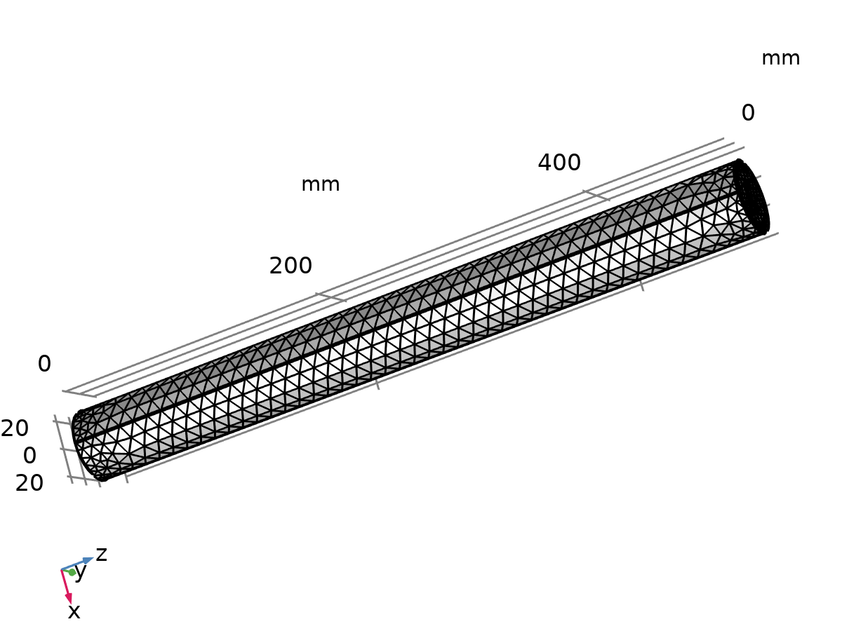
Voss clicked Compute. The iterative solver hummed across 71,792 degrees of freedom. In five seconds, the solutions converged.
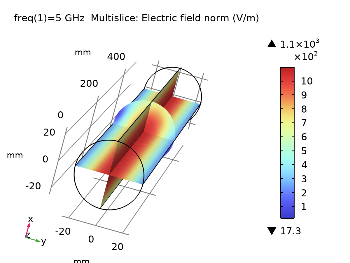
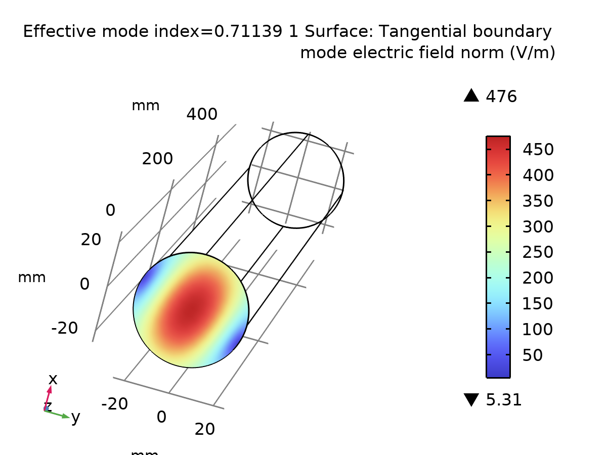
Download Original COMSOL Models (.mph) & Simulation Reports (.docx)
Explore and run the exact COMSOL Multiphysics models used in this study. The repository contains the full 3D boundary mode solvers, frequency domain studies at 5 GHz, mesh convergence setups, and complete Word (.docx) technical report generators for both modes:
WG_TE11.mph
📦 WG_TM01.mph
📄 WG_TE11.docx
📄 WG_TM01.docx
Theory vs. Numerical Reality
Kira pulled the numbers from the COMSOL post-processing derived tables (Phase Velocity, Wave Impedance, Emax, and Pmax) and laid them side-by-side with their analytical pencil-and-paper derivations.
| PARAMETER | THEORETICAL DERIVATION | COMSOL SIMULATION (PRACTICAL) | PERCENTAGE ERROR (%) | PHYSICAL SIGNIFICANCE |
|---|---|---|---|---|
| MODE 01: TRANSVERSE ELECTRIC (TE11) — DOMINANT MODE | ||||
| Cutoff Frequency (fc) | 3.5159 GHz | 3.516 GHz (seeded) | 0.00% | Fundamental cutoff; lowest frequency allowed into the conduit. |
| Effective Mode Index (neff) | 0.71101 | 0.711389 | 0.053% | Eigenvalue of boundary mode solver; determines wave reduction. |
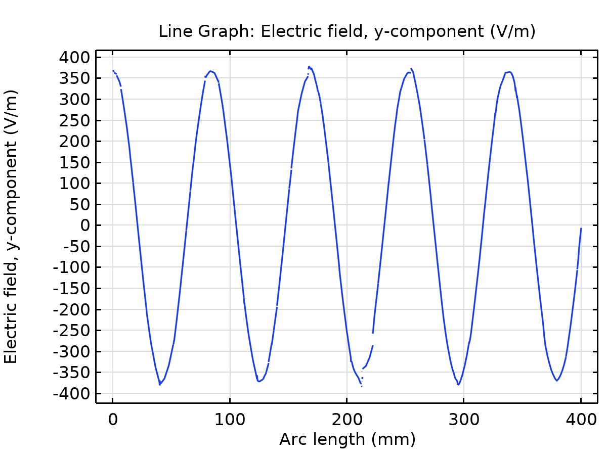
| Phase Velocity (vp) | 4.2194 × 10⁸ m/s | 4.2142 × 10⁸ m/s | 0.123% | Speed of crests along z; verified by line graph λg × 5 GHz. |
| Wave Impedance (ZTE) | 530.244 Ω | 529.570 Ω | 0.127% | Higher than free space (377 Ω); creates reflection at coax feed. |
| Guide Wavelength (λg) | 84.39 mm | 84.28 mm | 0.130% | Spatial distance between consecutive crests along conduit axis. |
| Peak Power Handling (Pmax) | 7.9552 MW | 7.0960 MW (Mesh Emax = 1126.3 V/m) | 10.80% | Air breakdown at 3 MV/m. Difference arises from boundary element curvature discretization. |
| Port Reflection (S11) | -∞ dB (Ideal match) | -87.45 dB | — | Outstanding transmission fidelity; virtually zero numerical reflections. |
| MODE 02: TRANSVERSE MAGNETIC (TM01) — HIGHER-ORDER MODE | ||||
| Cutoff Frequency (fc) | 4.5932 GHz | 4.593 GHz (seeded) | 0.00% | Second mode allowed; requires higher energy to propagate. |
| Effective Mode Index (neff) | 0.39503 | 0.396663 | 0.413% | Steeper cutoff factor; wave moves close to cutoff limit. |
| Phase Velocity (vp) | 7.5930 × 10⁸ m/s | 7.5579 × 10⁸ m/s | 0.462% | Superluminal phase speed; outruns TE11 by nearly a factor of 2. |
| Wave Impedance (ZTM) | 148.951 Ω | 149.430 Ω | 0.321% | Lower than free space (377 Ω); requires inductive tuning. |
| Guide Wavelength (λg) | 151.86 mm | 151.16 mm | 0.461% | Much longer spatial period along z due to high phase speed. |
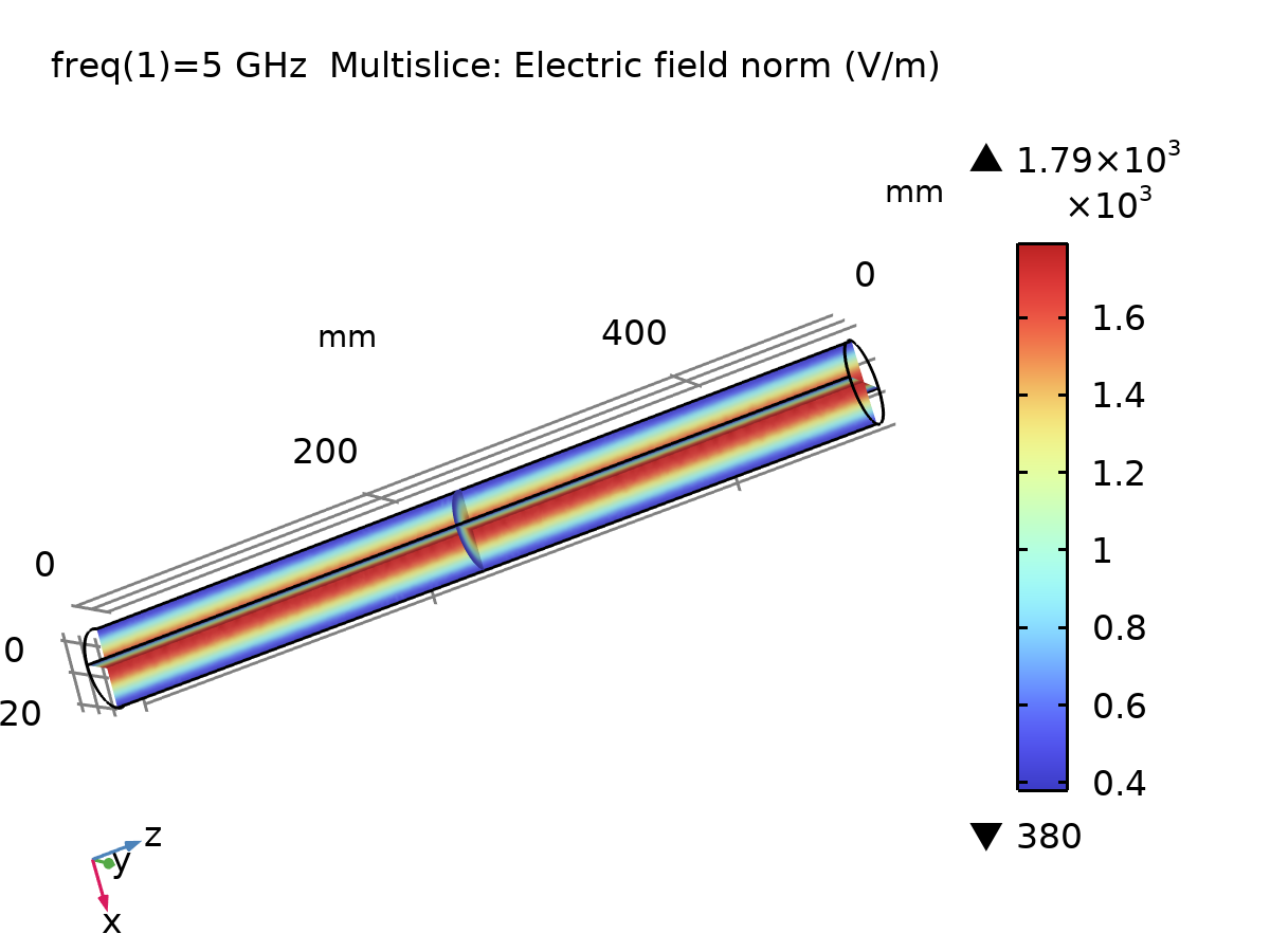
| Peak Power Handling (Pmax) | 2.9567 MW | 2.7336 MW (Mesh Emax = 1814.5 V/m) | 7.55% | Air breakdown at 3 MV/m. Centerline concentration triggers breakdown earlier than TE11. |
| Port Reflection (S11) | -∞ dB (Ideal match) | -69.91 dB | — | Negligible reflection at numerical receiving boundary. |
"Look at those numbers, Voss! 0.05% error on the effective index. 0.12% on the phase velocity. 0.13% on the impedance. The physical simulation didn't just match our Bessel series—it proved that our indicial equations captured the exact electromagnetic reality inside the metal."
"The only discrepancy appears in peak power capacity—a 7 to 10 percent variance. That is not an error in theory; it is the physical artifact of tetrahedral discretization. In pure theory, the Bessel function is perfectly smooth. In a finite-element mesh, piecewise quadratic polynomials approximate the cylindrical arc, producing slight localized field spikes that predict breakdown slightly sooner than ideal calculus."
The Turn in the Corridor
Kira stepped back from the console. The simulated pulses traversed the 500-millimeter tube with serene mathematical perfection. Every mode had been mapped. Every cutoff verified. Every power threshold calculated.
"Voss... we have mastered the straight pipe. We know how it breathes, how it chokes, and where it arcs. But real machines aren't straight. In a radar pedestal, a satellite transceiver, or an accelerator vault, signals can't travel in a straight line forever. To steer this RF energy into an antenna or around a reactor shield... the pipe has to bend."
Voss paused, his expression growing tense. He reached over to the CAD engine and swept the mouse, bending the straight cylindrical axis into a ninety-degree circular arc.
"A waveguide bend. When you curve the conduit, you shatter the cylindrical symmetry. The inner wall is shorter than the outer wall. The path length splits. The Bessel functions warp into complex toroidal coordinates, and the pure TE11 mode begins to couple into parasitic modes—scattering energy, creating phase distortion, and throwing reflections back down the throat of the generator."
"Then that is our next battle. Let's curve the pipe."
Original Notes — All 12 Pages Combined
Both Part 1 (Mode Topologies, High-Pass Action, Overmoding, C-Band Analytical Calculations, and Breakdown Limits) and Part 2 (COMSOL Pre-Processing, Boundary Mode Seeding, and Post-Processing Verifications) are combined into this unified 12-page interactive high-resolution viewer.